CENG 589 Digital Geometry Processing - 2 PCA

Introduction
In this assignment, our job was:
- Reading a database of different meshes that have the same topology
- Calculating an orthogonal basis using the database
- Synthesizing new shapes by altering the data in the direction of vectors that we have calculated
This process is called PCA(Principle Component Analysis). PCA has other applications such as dimension reduction and oriented bounding box computation.
Dependencies
For this task, I needed a linear algebra library. For that, I have included Eigen and Spectra. These libraries are header only so they were easy to include and use. I needed:
- Eigen for matrix operations.
- Spectra for calculating eigenvalues and eigenvectors of matrices.
Additional Classes
For this assignment, I have modified my codebase and added some new classes. These new classes are:
- Model Database: This class is responsible for collecting all the mesh objects' vertices and indices.
- PCA Database: This class uses the data in Model Database and is responsible for making calculations on it. It holds an Editor Mesh instance and this object is being drawn every frame. In addition it holds eigenvectors that are calculated in the constructor and their corresponding weights. If there is a change in some of the weights, an update function is triggered and therefore, we synthesize new meshes in real-time.
PCA Computation
To compute PCA, we first have to compute the mean of all samples. It is being done like the following:
Eigen::MatrixXd PCADatabase::CalculateMeanVertices()
{
    m_VertexSize = m_ModelDatabase->GetVertexCount();

    // Declare a column matrix for the mean
    Eigen::MatrixXd m = Eigen::MatrixXd::Zero(m_VertexSize * 3, 1);

    m_MeanVertices.resize(m_VertexSize, glm::vec3(0.0f));

    uint32_t sampleCount = m_ModelDatabase->GetMeshCount();

    std::vector<MeshBlueprint> meshes = m_ModelDatabase->GetMeshes();


    for (uint32_t i = 0; i < sampleCount; i++)
    {

        for (uint32_t j = 0; j < m_VertexSize; j++)
        {

            m(j*3, 0)     += meshes[i].vertices[j].x;
            m(j*3 + 1, 0) += meshes[i].vertices[j].y;
            m(j*3 + 2, 0) += meshes[i].vertices[j].z;
            m_MeanVertices[j] += meshes[i].vertices[j];
        }
    }

    for (uint32_t i = 0; i < sampleCount; i++)
    {
        m_MeanVertices[i] /= sampleCount;
    }

    m = m / sampleCount;

    GP_TRACE("Mean Vertex Calculation has finished");

    return m;

}
Indices are also important. One thing to notice is that indices do not change in the database. So, every object in the database has the same indices. We also acquire these indices. And then, we need to construct a Y matrix that has every database object's all vertices in its columns. So, for example, if we have a database with 1000 objects and each object has 2000 vertices. Our matrix will have 6000 rows and 1000 columns.
We also have to subtract the mean from each column of this matrix. It has to be like:
The matrix is being constructed with this function:
Eigen::MatrixXd PCADatabase::ConstructYMatrix(Eigen::MatrixXd mean)
{
    uint32_t sampleCount = m_ModelDatabase->GetMeshCount();

    Eigen::MatrixXd yMatrix(m_VertexSize * 3, sampleCount);

    std::vector<MeshBlueprint> meshes = m_ModelDatabase->GetMeshes();

    for (uint32_t i = 0; i < sampleCount; i++)
    {
        for (uint32_t j = 0; j < m_VertexSize; j++)
        {
            yMatrix(j * 3, i)     = meshes[i].vertices[j].x;
            yMatrix(j * 3 + 1, i) = meshes[i].vertices[j].y;
            yMatrix(j * 3 + 2, i) = meshes[i].vertices[j].z;
        }

        yMatrix.col(i) -= mean;
    }

    return yMatrix;
}
Later, we have to compute the the scatter(covariance) matrix. This matrix is simply
At last, we find have to find the Eigenvectors of S because these eigenvectors will give the directions that are very effective if we travel across it to synthesize models that have the highest variance. As we can notice, matrix S is symmetrical, dense and has a size of 3 times the vertex count squared. So, if each sample has 2000 vertices and 1000 samples, the size s of this matrix will become:
This is a huge matrix. This means it has a lot of eigenvalues and calculating these values is very hard. However, we, fortunately, have a way to lower the size. In our lectures, we have learned that with Karhunen-Loeve Transform, we can lower the size of this matrix to sample count squared rather than the size above. So, our size will become:
So we, change the Scatter matrix to this:
In my implementation, I calculate n-2 eigenvectors. So in the case above, I calculate 998 eigenvectors and eigenvalues. However, I do not use all of these eigenvectors. Most of these eigenvalues have negligible eigenvalues so they are not very important. I first find the sum of all eigenvalues. Secondly, I start iterating eigenvectors and look at their eigenvectors specifically and gradually add them. If this added value starts being higher than 90% of the original eigenvalue sum, then I stop the iteration. This way, I end up using 4-6 eigenvectors. However, these eigenvectors are not the eigenvectors of our real scatter matrix. To retrieve them, we multiply these eigenvectors with the Y matrix:
Here, pi is the eigenvector that we are interested in and qi is the eigenvalue of the small scatter matrix we constructed using Karhunen-Loeve Transform.
The code below shows everything that I have written above (in my implementation, it is the constructor of PCADatabase class):
PCADatabase::PCADatabase(Ref<ModelDatabase> modelDB) : m_ModelDatabase(modelDB)
{
   GP_TRACE("Size of database is: {0}", m_ModelDatabase->GetMeshCount());
   m_Indices = m_ModelDatabase->GetIndices();

   // Get mean vector
   GP_TRACE("Mean Vector Calculation");
   Eigen::MatrixXd mean = CalculateMeanVertices();
   m_Mean = mean;

   // Get Y Matrix
   GP_TRACE("Y matrix Calculation");
   Eigen::MatrixXd yMatrix = ConstructYMatrix(mean);

   // Karhunen-Loeve Transform
   GP_TRACE("Scatter Calculation");
   Eigen::MatrixXd kScatter = yMatrix.transpose() * yMatrix;

   // Construct matrix operation object using the wrapper class DenseSymMatProd
   Spectra::DenseSymMatProd<double> op(kScatter);

   GP_TRACE("EigenValue Calc");
   int meshCount = m_ModelDatabase->GetMeshCount();
   Spectra::SymEigsSolver<Spectra::DenseSymMatProd<double>> eigs(op, meshCount - 2,
                                                                       meshCount);
   eigs.init();
   int nconv = eigs.compute(Spectra::SortRule::LargestAlge);

   // Retrieve results
   Eigen::VectorXd evalues;
   Eigen::MatrixXd eigenVectors;
   if (eigs.info() == Spectra::CompInfo::Successful)
   {
       evalues = eigs.eigenvalues();
       eigenVectors = eigs.eigenvectors();
   }

   float evalueSum = evalues.sum();

   // Now compute real eigenvectors
   float totalEvalue = 0.0f;
   for (uint32_t i = 0; i < eigenVectors.cols(); i++)
   {
       float currentEvalue = evalues(i);
       totalEvalue += currentEvalue;

       if (totalEvalue / evalueSum >= 0.9)
           break;

       m_Eigenvectors.push_back(yMatrix * eigenVectors.col(i));
       m_Coeffs.push_back(0.0f);
   }

   // Calculate new vertices
   Eigen::MatrixXd x = m_Mean;
   for (uint32_t i = 0; i < m_Eigenvectors.size(); i++)
   {
       x += m_Eigenvectors[i] * m_Coeffs[i];
   }

   for (uint32_t i = 0; i < x.rows(); i+=3)
   {
       m_Vertices.push_back(glm::vec3(x(i,0), x(i + 1, 0), x(i + 2, 0)));
   }

   // Construct mesh
   m_EditorMesh = EditorMesh::Create("Test", m_Vertices, m_Indices);
}
Lastly, since we have our eigenvalues and mean. We need to linearly map them like the following:
This is a linear correlation. This way, we synthesize new shapes.
Further investigation and Experiments
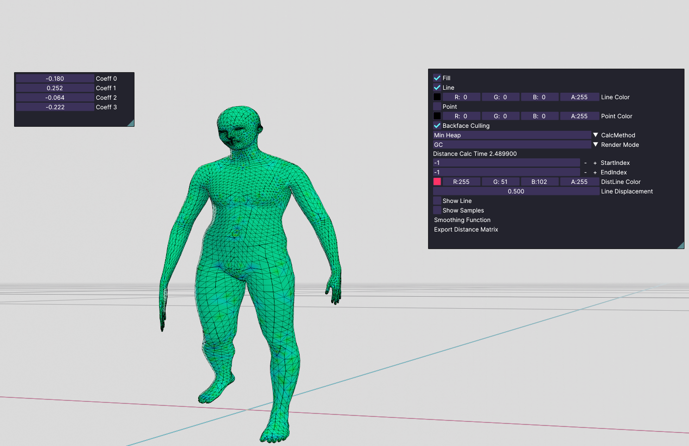
After implementing these, I started experimenting. First of all, I used the dataset I took from Semantic Parametric Reshaping of Models which is derived from CAESAR dataset. It has human bodies that have different physical characteristics. First of all, I would like to share a video where I play around with the coefficients of eigenvectors. Each coefficient seems to change a certain characteristic of the shape. For example, It seems like the first coefficient changes the height of the shape:
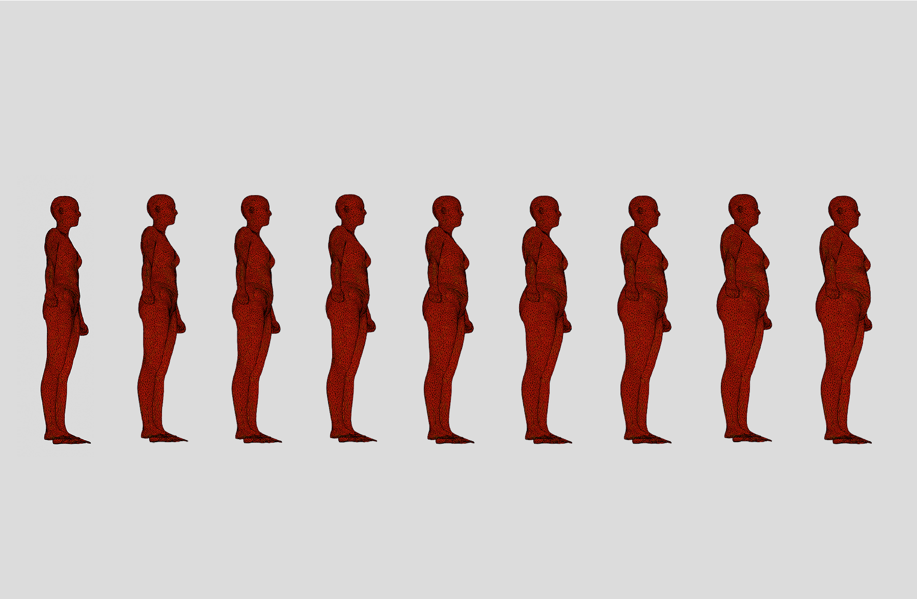
I have also merged these different shapes and saw a spectrum of characteristics. For example, in the image below, I am only changing the first coefficient and this is how it looks like:
height change
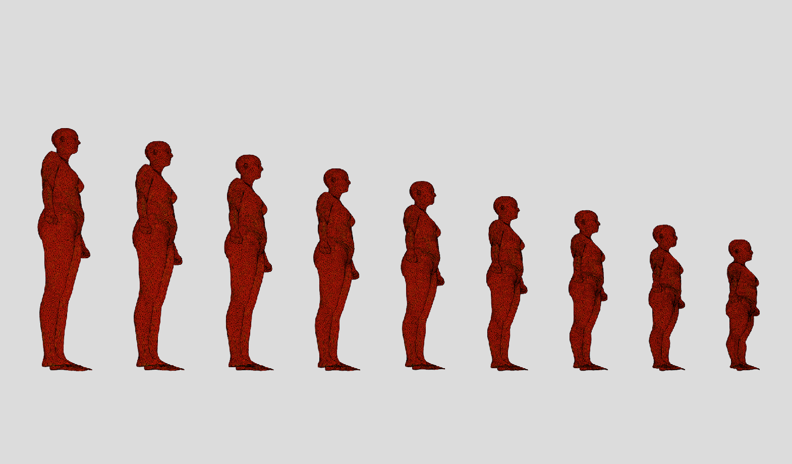
Here is another example of when I started playing around only with component 3. It seems to affect the weight of the body:
weight change
After playing around with this database, I have downloaded another dataset named FAUST. Unlike the other one, this dataset contains characters with different poses. This is the mean shape I get:
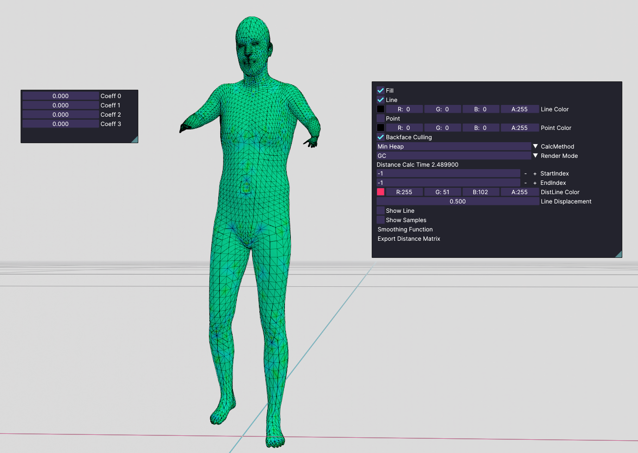
mean shape
We see that this person's hands look like a t-rex. So, I started playing around with only one coefficient at a time. I saw that none of them are meaningful by themselves. But I got pretty much-distorted bodies. But If I started tweaking all coefficients at the same time, I started getting meaningful poses. For example:
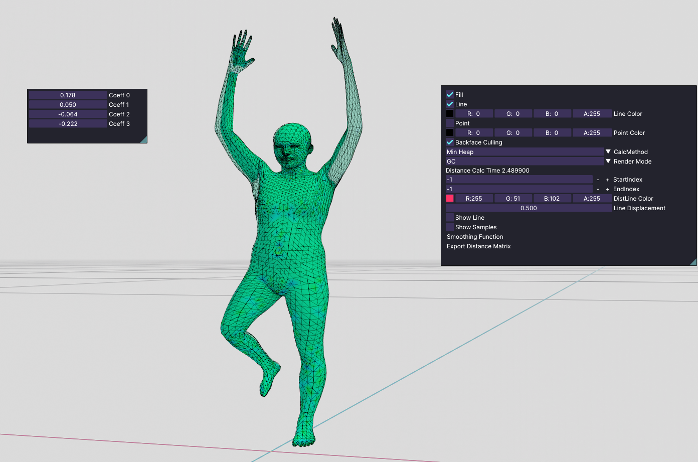
pose 1
Here is another pose:
pose 2
These poses are still looking distorted, but It proves that the eigenvectors of this dataset are not meaningful if they are alone.
Non-Linear Correlation
So, this means that for this dataset, we need something like a nonlinear correlation. For example, there will be weights for different poses and these weights will be mapped to the weights of all eigenvectors. I think it looks like neural networks. Our poses will be the inputs and the outputs are the coefficients of the eigenvectors. But, for this, I need a dataset to train which has true classes. Since I could not find a dataset like this, I could not use a non-linear correlation.
I'm not exactly sure what I have come up with the thing I wrote above but this is how I observed and it might be wrong.
Conclusion
This was the second assignment for the Digital Geometry Processing course. Since I implemented my own mesh viewer in the first assignment, this time, It was easier for me to solve this assignment because I have full control over my source code. As I shared before, the link above is the repository of this mesh viewer of mine: