CENG 589 Digital Geometry Processing
Introduction
Since I'm already implementing my own game engine and trying to improve as a graphics programmer thanks to brilliant content creators and authors on the internet such as TheCherno, Inigo Quilez, Joey de Vries, Etay Meiri and so many others.
Normally, I had to use existing 3D viewers and directly implement the assignment. Thus, the first assignment, I could not finish it in time. But I got a 3D mesh viewer that renders a model with different rendering and coloring modes and an orbital camera that is controlled with the mouse. I first want to explain what this mesh editor does and how it works. I am not going to get into details how I got this editor up and running from scratch because that is not the topic of the journey. However it was the hardest part.
File Structure of the Executable
This application uses Assimp as a dynamic library for loading different models. If we consider the folder that the executable resides as the root folder. We store the assets in a folder called assets. The structure of assets folder looks like the following.
- Assets
- fonts: Fonts that are used for Imgui are stored here
- models: All models are stored here, they are all loaded at startup.
- output: For assignment1, we need to export a geodesic distance matrix. This folder holds these matrices.
- shdaders: All shaders that are used for visualization are kept here.
- include: Shader includes
- src: Shader sources
- textures: For now, It keeps the environment maps.
Runtime
When we first open the executable, a scene with a whiteish environment map opens. For now, a hard-coded model is directly loaded (I will change it in a couple of days). When a model is loaded, these happen:
- Vertices, Normals, TexCoords and Indices are read using Assimp.
- Triangles are determined for calculating their qualities in the future.
- Setting up flat vertices and normals. We need this because for coloring individual triangles, we need flat shading. This is the solution I found but there might be better solutions.
- Setting up the node table that we use for calculating dijkstra's shortest path between vertices. We also have another node table for calculating the NxN Geodesic distance matrix. Node tables are unordered maps.
- Set up the adjacency map, for getting neighbors of vertices. We need this in multiple places.
- Setting up tangents and bitangents. Honestly, we do not need it for now, because we do not deal with textures. But I calculate them anyways.
- Calculating colors for assignment. We compute colors for Gaussian Curvature, Average Geodesic Distance and Triangle Quality
- We set up different vertex array objects for coloring. Instead of filling the same buffer every frame, I decided to keep multiple buffer objects and switch them when the rendering mode changes.
- Lastly, we set up the main vertex array object.
The image below shows the GUI and the scene when we first open the executable:
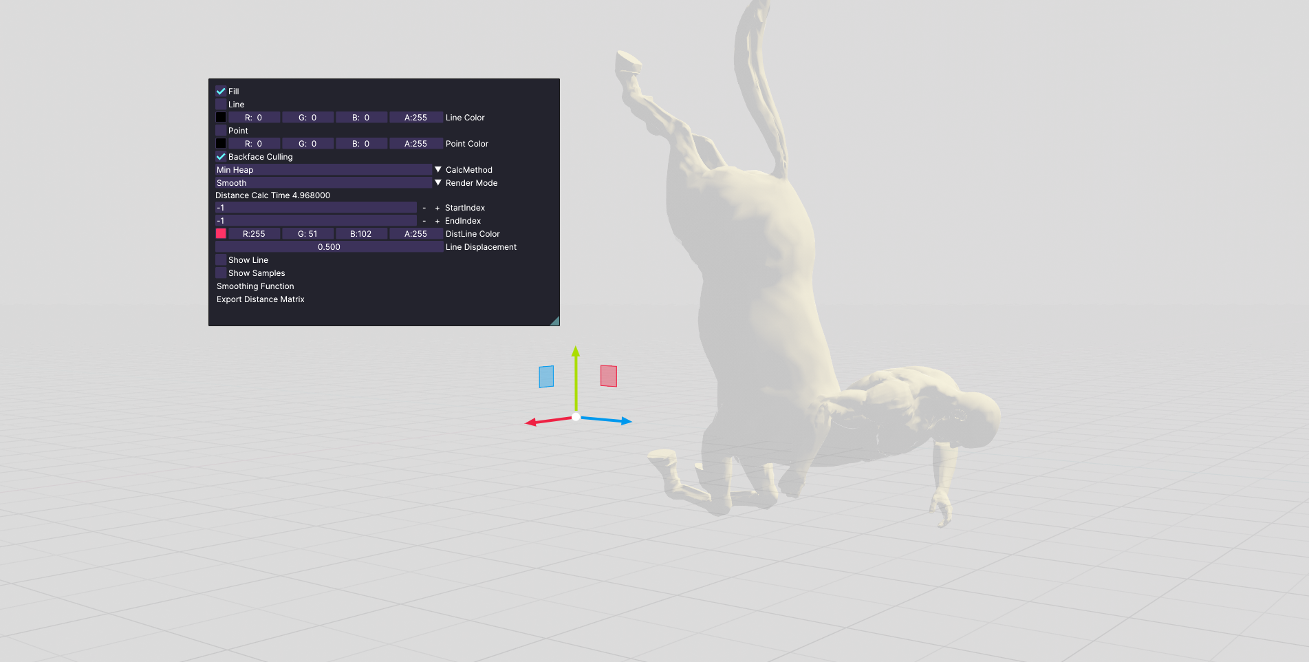
Editor at Startup
As is seen here, this application uses Dear ImGui as a GUI library. There are two windows, one is the viewport and the other is the window for settings. In the viewport, we see a scene with an infinite grid and a weirdly oriented centaur for now. The reason is the initial coordinates of the centaur are flipped on their y and z-axis. We also see a gizmo for moving the object. We can use it with our mouse. There are different modes of manipulating transform of the mesh:
- Hiding Gizmo: When Q is pressed, the gizmo is hidden.
- Translation: When W is pressed, the gizmo changes its mode to the translation mode
- Rotation: When E is pressed, the gizmo changes to the rotation mode
- Scale: When R is pressed, the gizmo changes to the scaling mode.
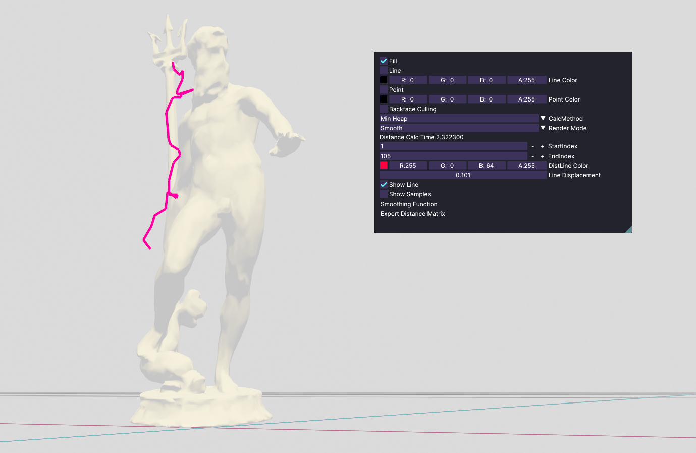
In the settings window there are different checkboxes, color pickers, combo boxes and input places. They do the following:
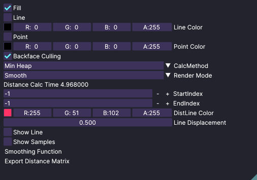
Settings Window
- Fill: When it is selected, we can see the whole object in fill mode.
- Line: Object is rendered as lines.
- Line Color: We can change the line color.
- Point: Object is rendered as points.
- Point Color: We can change the point color.
- Backface Culling: Toggles backface culling option.
- Calc Method: This combo box decides which data structure we use for dijkstra's shortest path algorithm.
- Render Mode: This combo box decides the rendering mode when fill is enabled. These modes are:
- Average Geodesic Distances
- Flat shading
- Gaussian Curvature
- Triangle Quality
- Smooth shading
- Calculation Time: This text area shows the time that is passed while calculating dijkstra's shortest path in milliseconds.
- Start and End Indices: These two fields are used for drawing the shortest line which connects two vertices along the surface of the mesh.
- Line Color: Color of the line determined below.
- Line Displacement: Sometimes, lines might overlap with the surface. This displacement factor transforms the vertices of the line in direction of the surface normal.
- Show Line: Toggles showing lines.
- Show samples: For average geodesic distance calculations, we sample points on the mesh. This is for visualizing these points. Spheres are used for this.
- Smooting Function: This function smoothes the mesh by moving each vertex towards the center of all one ring neighbors. I saw that using this multiple times increases triangle qualities.
- Export Distance Matrix: When this button is clicked, geodesic distance matrix is exported to the output folder with the name of the mesh. It is done asyncronously using future and async.
Geodesic Distance Calculation
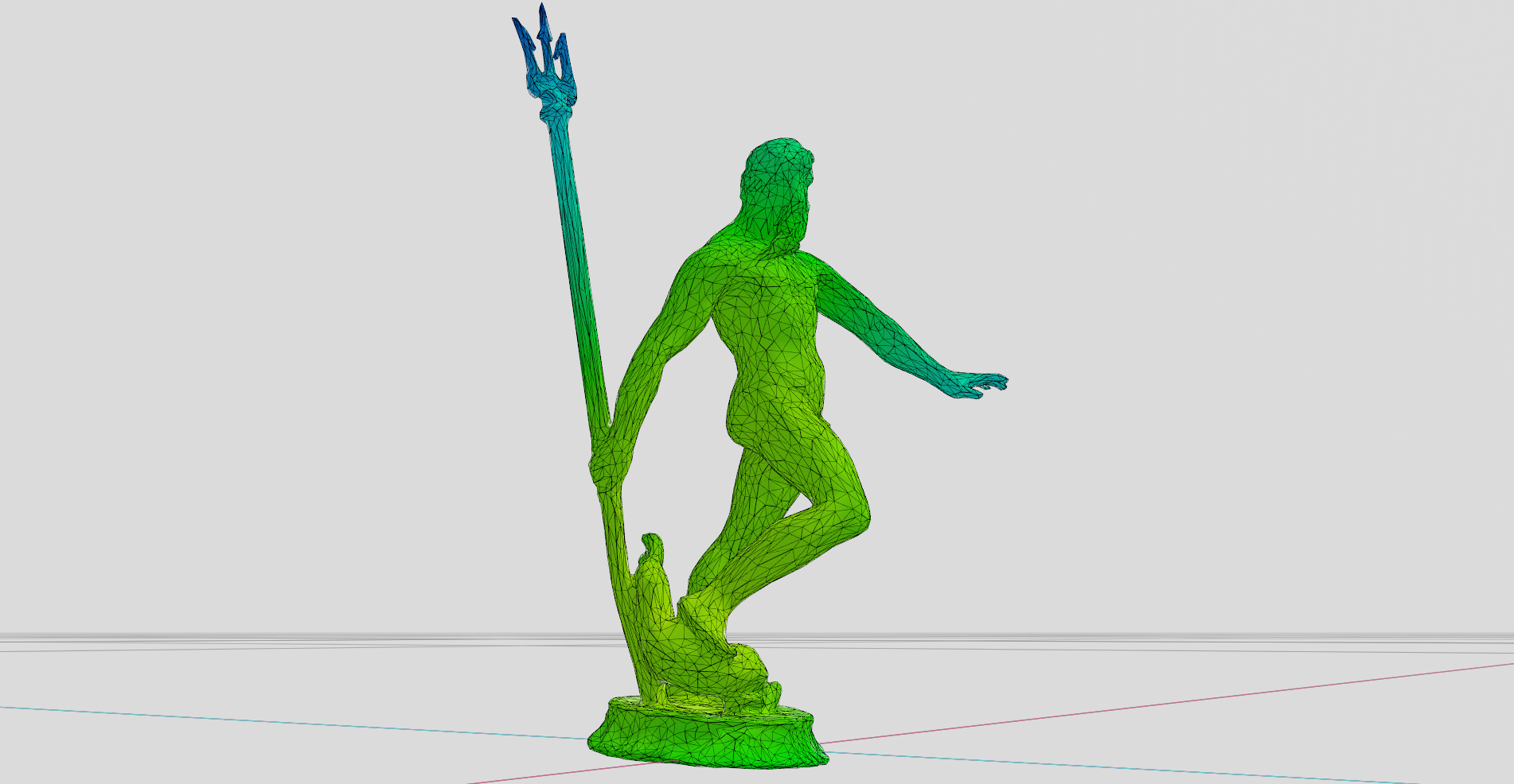
In the first part of the assignment, we have to select two vertices on the mesh and visualize the shortest geodesic path between them. We also need to report the timings for different data structures. We had to do that for array, min heap and fibonacci heap. But I could not implement fibonacci heap for now. But I know that fibonacci heap is more efficient in theory and not so efficient as min heap in practice. For demostration, I have loaded neptune model and explain everything using this model from now on.
The image below shows the geodesic distance between points with indices 1 and 105. This can be changed from the settings window and it shows the path right away. In this case, the first vertex is the one on below.
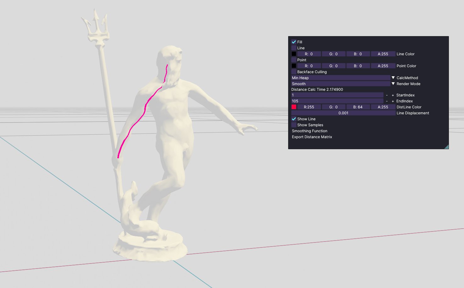
Geodesic Distance 1
One thing here to note is that the line displacement. This is set as 0.001 but it is just for this model. There are other models where the scale is much bigger. So we for these we need bigger line displacements for better visualizations. For example, if we increase line displacement, we get this:
Wrong Line Displacement
We see that the line is displaced a lot. So we have to choose this factor accordingly.
Secondly, we see that when we start playing around with indices, we immediately see the time needed for that geodesic distance calculation. We can also select different data structures and compare their values. In my case, min heap was significantly faster than array. This is understandable because min heap is a priority queue and it is easier to get minimum values instead of searching min value and erasing from array.
| Data Structure | Time |
|---|---|
| Min Heap | 2.013 ms |
| Array | 5.465 ms |
Lastly, when we press to Export Distance Matrix, we get the NxN Geodesic Distance matrix which shows closest distance from vertices to all other vertices. Matrix is saved under output folder as I have explained. For bigger meshes, it is harder to calculate so it takes a lot of time and space. For helping, I have implemented this functionality asyncronous. This way our rendering is not interrupted.
Descriptors and Sampling
In this part, we had to compute Gaussian Curvature and Average Geodesic Dsitance and assign smooth colors. Next, we also had to calculate the quality of each triangle and assign colors to them individually.
First, In the assignment, it is said that we have interpolate normalized values of descriptors from red, greed to blue. I have learnt that the best way to do such an interpolation is using hsv color space instead of rgb that I currently use. So my first job was searching for conversion functions between hsv and rgb. My plan was firstly compute the interpolated color using hsv (we only change the hue) and normalized value and secondly, converting it to the rgb color. Luckily, I was able to find one. This is the function by fairlight1337 I found on GitHub. Here is how I used it in my project:
static glm::vec3 Hsv2Rgb(glm::vec3 hsvColor)
{
    float fC = hsvColor.z * hsvColor.y;
    float fHprime = std::fmod(hsvColor.x / 60.0f, 6);
    float fX = fC * (1 - std::fabs(std::fmod(fHprime, 2) - 1));
    float fM = hsvColor.z - fC;

    glm::vec3 resultRgb;

    if (0 <= fHprime && fHprime < 1)
    {
        resultRgb = glm::vec3(fC, fX, 0.0f);
    }
    else if (1 <= fHprime && fHprime < 2)
    {
        resultRgb = glm::vec3(fX, fC, 0.0f);
    }
    else if (2 <= fHprime && fHprime < 3)
    {
        resultRgb = glm::vec3(0.0f, fC, fX);
    }
    else if (3 <= fHprime && fHprime < 4)
    {
        resultRgb = glm::vec3(0.0f, fX, fC);
    }
    else if (4 <= fHprime && fHprime < 5)
    {
        resultRgb = glm::vec3(fX, 0.0f, fC);
    }
    else if (5 <= fHprime && fHprime < 6)
    {
        resultRgb = glm::vec3(fC, 0.0f, fX);
    }
    else
    {
        resultRgb = glm::vec3(0.0f, 0.0f, 0.0f);
    }

    resultRgb += glm::vec3(fM, fM, fM);

    return resultRgb;
}
And the interpolation is simply this function:
static glm::vec3 GiveGradientColorBetweenRedAndBlue(float t)
{
    // A color between red and blue (passes from green in the middle)
    glm::vec3 hsvColor = glm::vec3(std::min(t, 1.0f) * 228.0f, 1.0, 0.6f);

    return Hsv2Rgb(hsvColor);
}
So, after solving this issue, I started implemented Gaussian Curvature first.
Gaussian Curvature
In our lecture slides, curvature is defined like the following:
So, according to the formula, we are just adding the angles in a one ring neighborhood and subtracting it from 2*pi. As I understood, we get much higher values when there are steeper curves. The image below shows the logic:
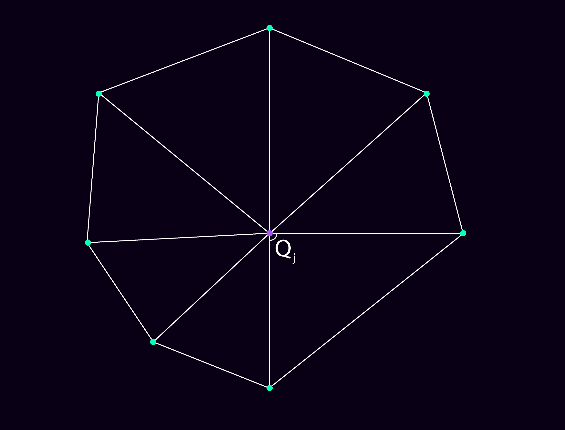
Gaussian Curvature
And this is how the coloring looks on model neptune:
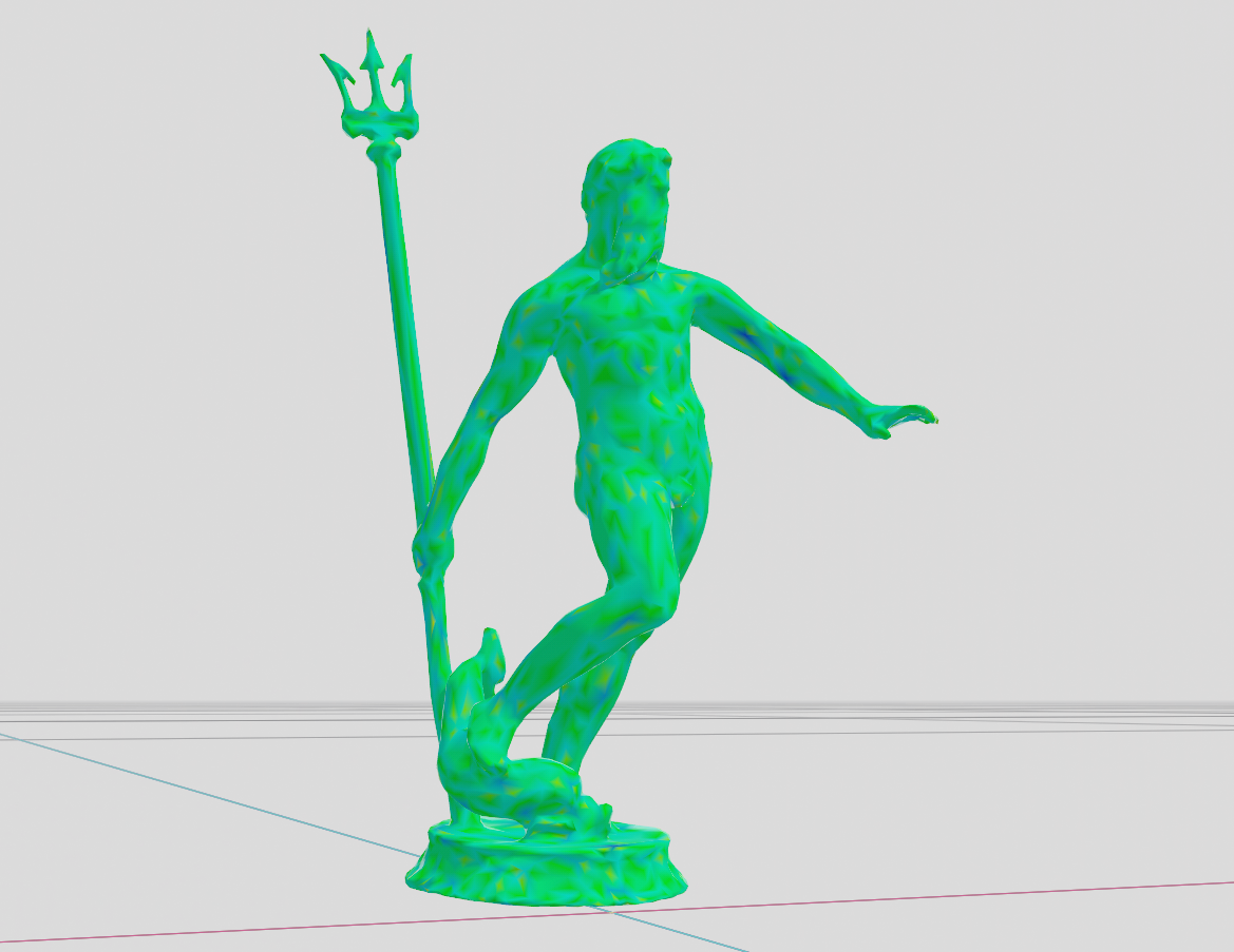
Gaussian Curvature: Neptune
Average Geodesic Distance
Next, we had to implement average geodesic distance for each vertex. Invoking dijkstra's shortest path algorithm everytime is not a good idea. So, we have to take some samples on the model. In the assignment, we have used FPS sampling which takes samples gradually. In this sampling method, we get the next sample by looking at what we have and remembering the closest vertex in the sample, we get the candidate which has the furthest away from the closest vertex in the sample set.
For getting distances, there are two options:
- Geodesic distances
- Euclidean distances
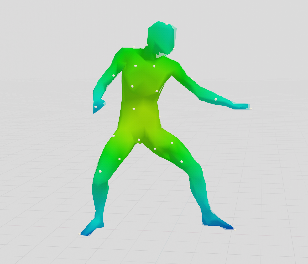
For simplicity, I am using a simpler model called man0 from now on. When Geodesic distances are used, we increase compute cost a lot because we have to compute a lot of shortest path algorithms. But we do not have this problem with euclidean distances. The problem with euclidead distances is that it does not consider the shape of the mdoel as I understood. So, let's experiment on them.
Let's get 500 samples using Euclidean distances. This is the Average Geodesic Distances colors and the samples.
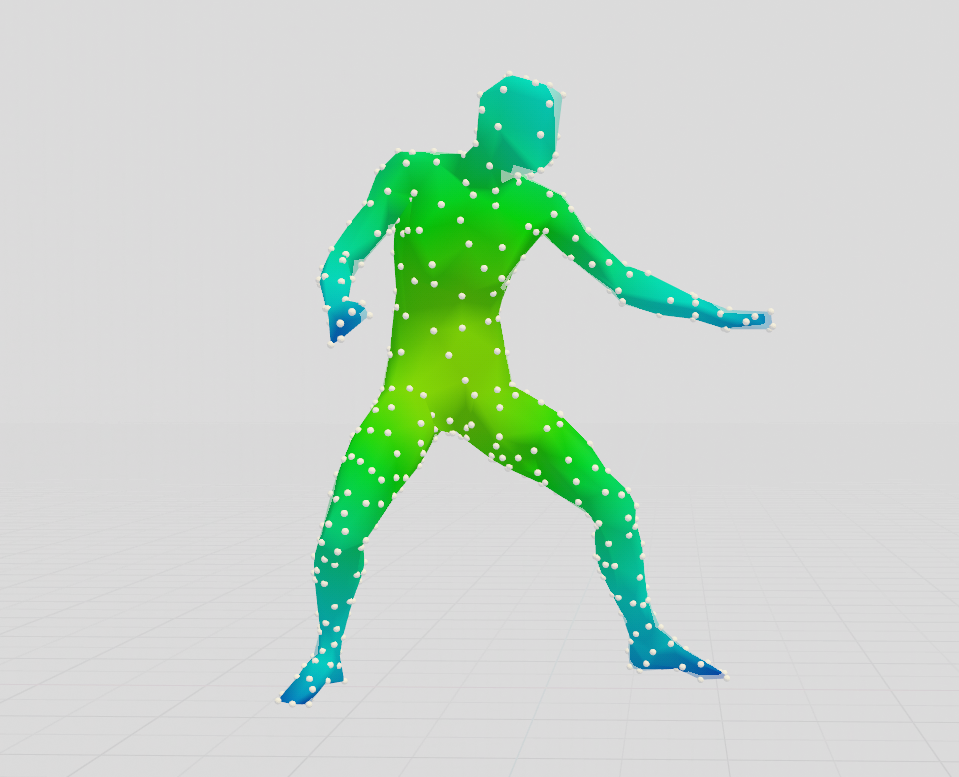
500 Samples Euclidean
We see that the samples are taken from reasonable places and the coloring seems ok. The more blue a place is, the more far away from the average of all other vertices. What happens if we lower the count of samples, to 50 maybe?
50 Samples Euclidean
It is still pretty much consistent. Now' lets do it with geodesic distances and 20 samples.
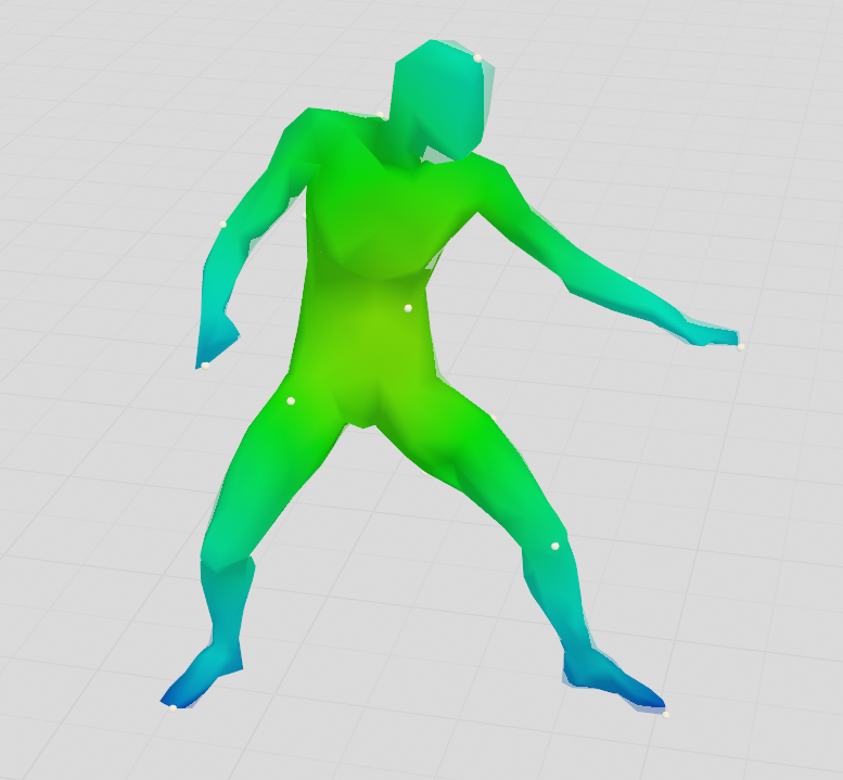
20 Samples Geodesic
It is still ok. However, with geodesic distances, we lose a lot of computational time. The euclidean is much better for performance by losing from accuracy a bit. And the model I'm using is also not very complex. Geodesic distance usage might be better for more complex objects.
Triangle Quality
Now, we have to compute each triangle's quality. Quality is associated with the ratio of circum-radius(radius of the smallest circle around the triangle) and the shortest edge of the triangle. The formula for circum radius is:
In this formula, A is the area of the triangle and it is computed by taking cross product of two edges , dividing it by 2 and taking its absolute value.
By using this knowledge, we can now do the coding and see the qualities of triangles. The higher the number is, the quality decreases. So, in our case, triangles with bad quality will be more blueish and high quality triangles will be reddish. For this, I want to use cat model. Let's look at the quality of triangles.
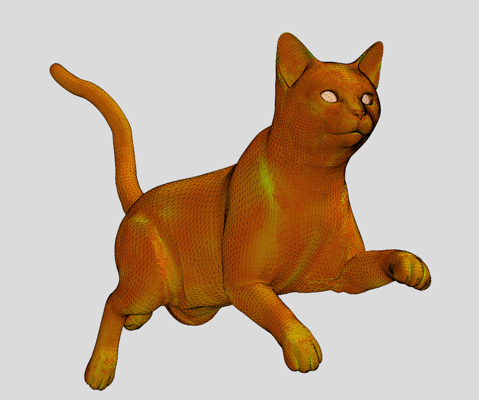
Cat Triangle Quality
As we can see above, most of the model's triangles are in good shape. But there must be some bad quality triangles especially in places like paws. I want to zoom into the right paw of the cat, because I spotted some bad quality triangles there. If we zoom into the leftmost nail of the cat on the right paw, that's what we see:
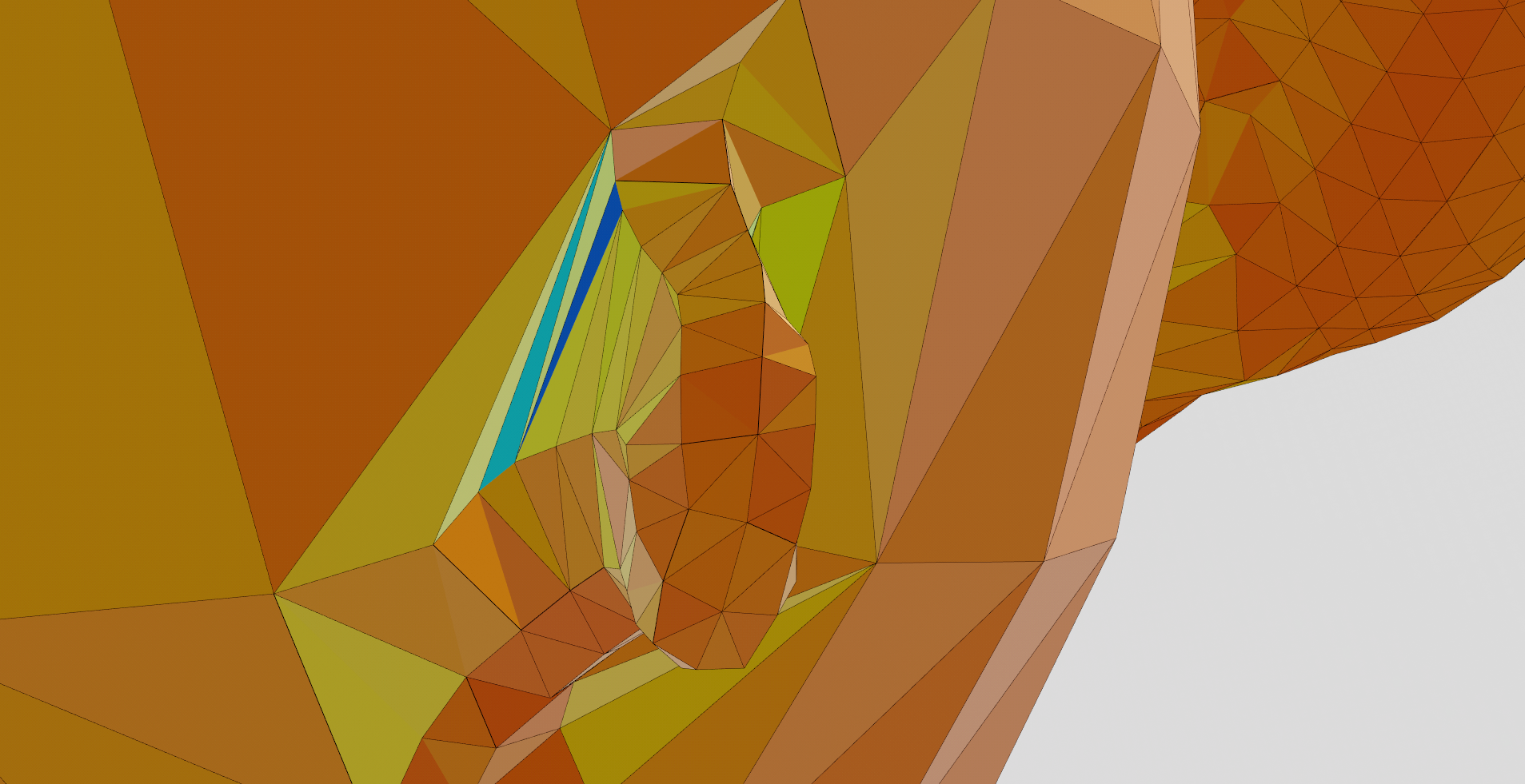
Cat Triangle Quality Paw
So, we see two bad quality triangles here and they are blue.
Smoothing Operation
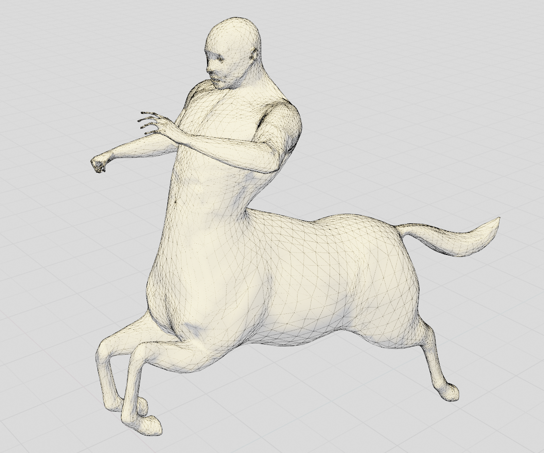
The last thing I did for this assignment was the smoothing function. We can trigger this function from the settings window. It moves each vertex towards the center vertex of all of the one-ring neighbors. Let's see how, Gaussian Curvature, Average Geodesic Distance and Triangle Qualities change when we apply this function like 20 times. For this, I want to use the centaur model.
First these images below are before the smoothing operation:
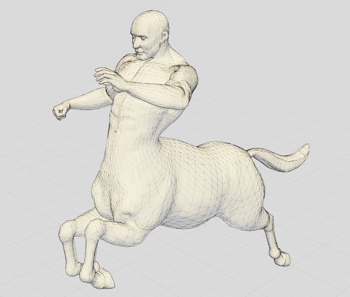
Smooth Shading Centaur
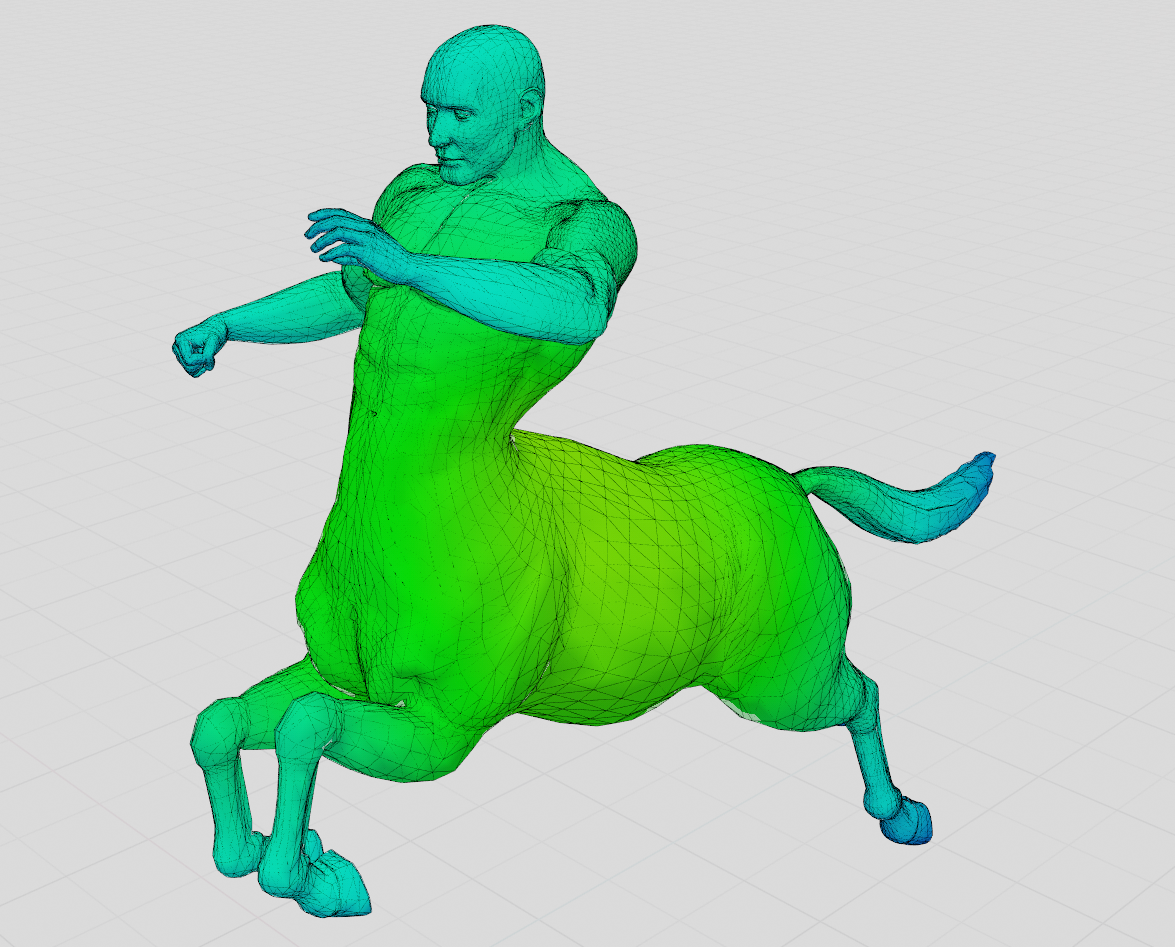
Average Geodesic Distance Centaur
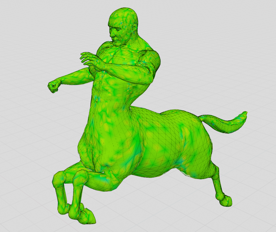
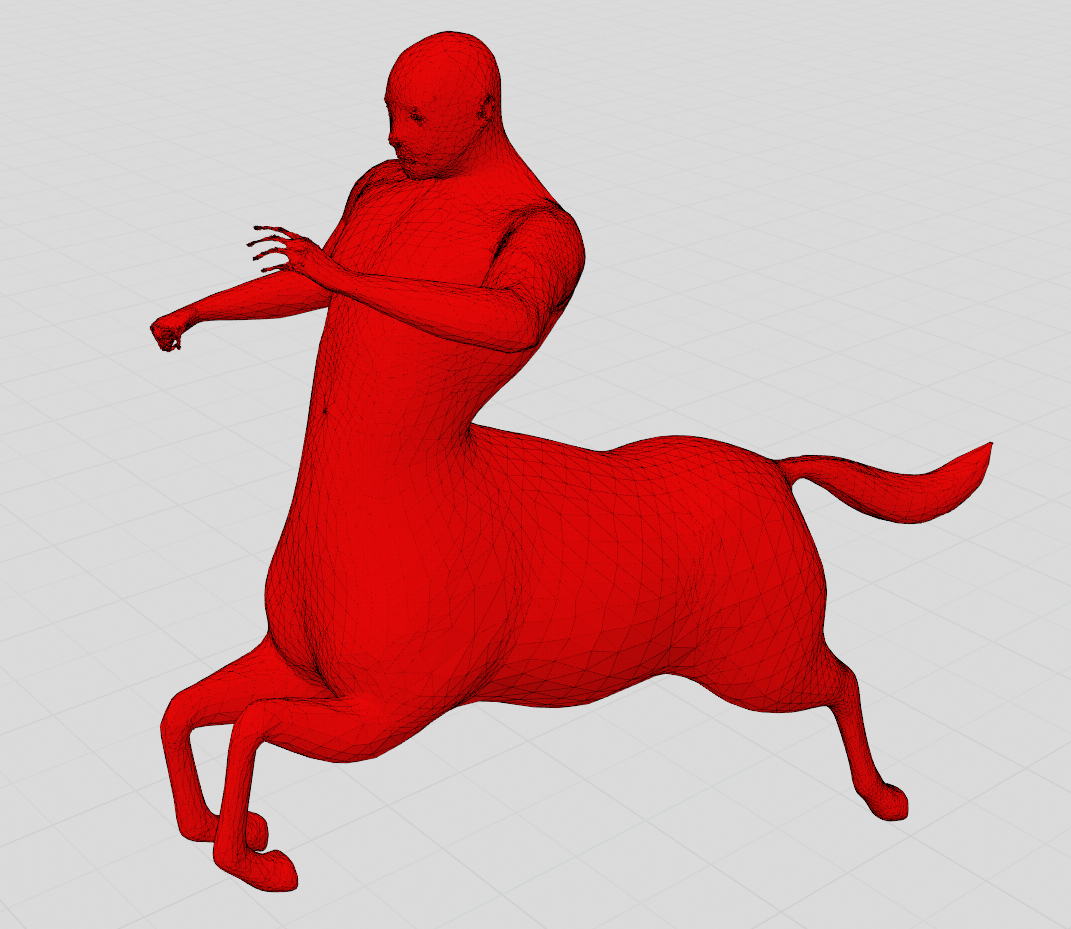
Gaussian Curvature Centaur
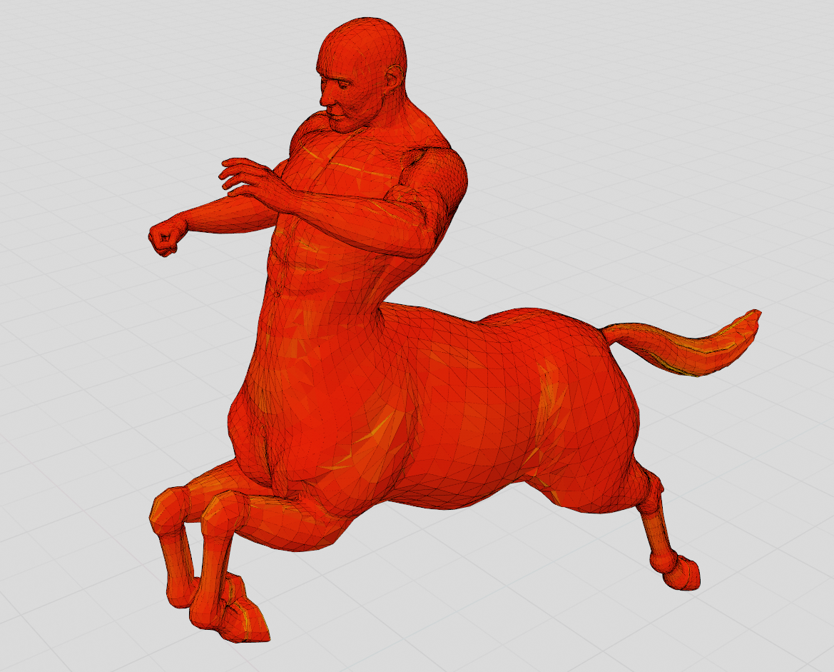
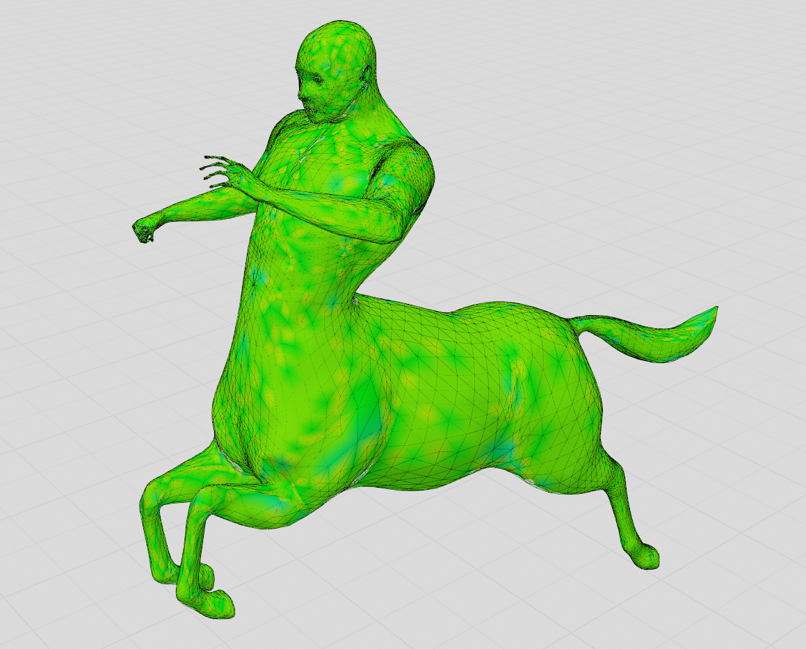
Triangle Quality Centaur
So this is the original centaur model. Now, I have applied smooth function 20 times. This is the result:
Smooth Shading Centaur 2
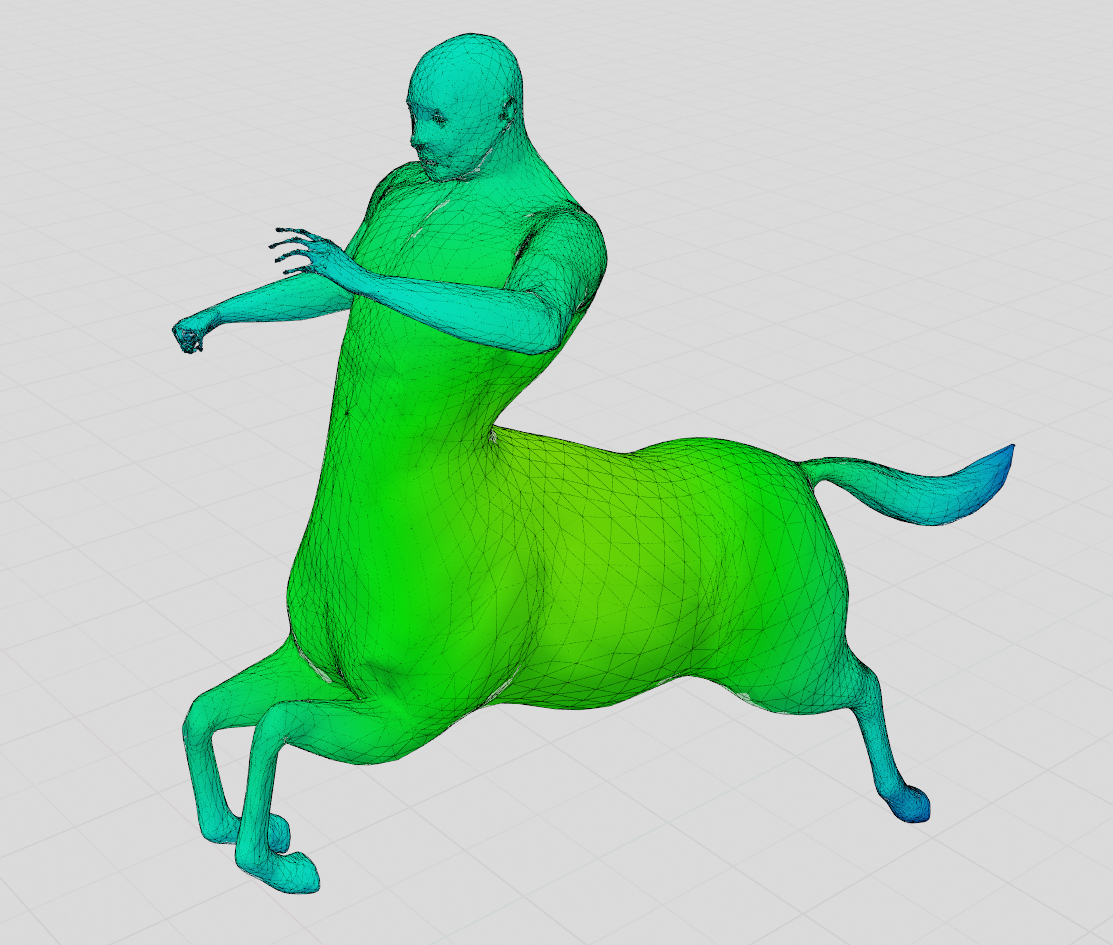
Average Geodesic Distance Centaur 2
Gaussian Curvature Centaur 2
Triangle Quality Centaur 2
The most significant change is for the triangle quality and the shape of the mesh. Mesh started collapsing and we can see the distortion. However, it increased the triangle quality overall. Actually, to get perfect triangles all over the mesh, just 2 or 3 smoothing operations were enough. After that, in some steps, triangle quailty worsened again but luckily, at the 20th step, I got a perfect triangle result again.
Conclusion
This was the first assigment for the Digital Geometry Processing Class. I plan to implement other tasks and projects using this application that I've built. It is hard to maintain it but this challenge helps me become a better graphics programmer. While first building this application from scratch, I have encountered a lot of graphics related problems and could not understand how to solve them. Fortunately, I became more familliar with RenderDoc and solved problems on my shaders. I know that RenderDoc is a widely used GPU profiler in the industry and I need to learn about it more.